Modeling relational event networks with remstimate

A tutorial

The aim of the function remstimate() is to find the set of model parameters that optimizes either: (1) the likelihood function given the observed data or (2) the posterior probability of the parameters given the prior information on their distribution and the likelihood of the data. Furthermore, the likelihood function may differ depending on the modeling framework used, be it tie-oriented or actor-oriented:

• the tie-oriented framework, which models the occurrence of dyadic events as realization of ties along with their waiting time (Butts 2008);

• the actor-oriented framework, which models the occurrence of the dyadic events as a two-steps process (Stadtfeld and Block 2017):

  1. in the first step, it models the propensity of any actor to initiate any form of interaction as a sender and the waiting time to the next interaction (sender rate model);
  2. in the second step, it models the probability of the sender at 1. choosing the receiver of its future interaction (receiver choice model).

The mandatory input arguments of remstimate() are:

• reh, which is a remify object of the processed relational event history (processing function remify available with the package remify, install.packages("remify"));

• stats, a remstats object (the remstats function for calculating network statistics is available with the package remstats, install.packages("remstats")). A linear predictor for the model is specified via a formula object (for the actor-oriented framework, up to two linear predictors can be specified) and supplied to the function remstats::remstats() along with the remify object. When attr(reh,"model") is "tie", stats consists of only one array of statistics; if attr(reh,"model") is "actor", stats consists of a list that can contain up to two arrays named "sender_stats" and "receiver_stats". The first array contains the statistics for the sender model (event rate model), the second array for the receiver model (multinomial choice model). Furthermore, it is possible to calculate the statistics for only the sender model or only the receiver model, by supplying the formula object only for one of the two models. For more details on the use of remstats::remstats(), see help(topic=remstats,package=remstats).

Along with the two mandatory arguments, the argument method refers to the optimization routine to use for the estimation of the model parameters and its default value is "MLE". Methods available in remstimate are: Maximum Likelihood Estimation ("MLE"), Adaptive Gradient Descent ("GDADAMAX"), Bayesian Sampling Importance Resampling ("BSIR"), Hamiltonian Monte Carlo ("HMC").

---

Estimation approaches: Frequentist and Bayesian

In order to optimize model parameters, the available approaches resort to either the Frequentist theory or the Bayesian theory. The remstimate package provides several optimization methods to estimate the model parameters:

• two Frequentist approaches such as Maximum Likelihood Estimation ("MLE") and Adaptive Gradient Descent ("GDADAMAX") which are respectively second-order and first-order optimization algorithms;
• two Bayesian approaches such as Bayesian Sampling Importance Resampling ("BSIR") and Hamiltonian Monte Carlo ("HMC").

To provide a concise overview of the two approaches, consider a time-ordered sequence of \(M\) relational events, \(E_{t_M}=(e_1,\ldots,e_M)\), the array of statistics (explanatory variables) \(X\), and \(\boldsymbol{\beta}\) the vector of model parameters describing the effect of the explanatory variables, which we want to estimate. The explanation that follows below is valid for both tie-oriented and actor-oriented modeling frameworks.

The aim of the Frequentist approaches is to find the set of parameters \(\boldsymbol{\hat{\beta}}\) that maximizes the value of the likelihood function \(\mathscr{L}(\boldsymbol{\beta}; E_{t_M},X)\), that is

\[ \boldsymbol{\hat{\beta}}=\mathop{\mathrm{arg\,max}}_{\boldsymbol{\beta}}\{\mathscr{L}(\boldsymbol{\beta};E_{t_M},X)\} \]

Whereas, the aim of the Bayesian approaches is to find the set of parameters \(\boldsymbol{\hat{\beta}}\) that maximizes the posterior probability of the model which is proportional to the likelihood of the observed data and the prior distribution assumed over the model parameters,

\[p(\boldsymbol{\beta}|E_{t_M},X) \propto \mathscr{L}(\boldsymbol{\beta}; E_{t_M},X) p(\boldsymbol{\beta})\]

where \(p(\boldsymbol{\beta})\) is the prior distribution of the model parameters which, for instance, can be assumed as a multivariate normal distribution,

\[ \boldsymbol{\beta} \sim \mathcal{N}(\boldsymbol{\mu_{0}},\Sigma_{0}) \]

with parameters \((\boldsymbol{\mu_{0}},\Sigma_{0})\) summarizing the prior information that the researcher may have on the distributon of \(\boldsymbol{\beta}\).

---

Let’s get started (loading the remstimate package)

Before starting, we want to first load the remstimate package. This will laod in turn remify and remstats, which we need respectively for processing the relational event history and for calculating/processing the statistics specified in the model:

library(remstimate)

In this tutorial, we are going to use the main functions from remify and remstats by setting their arguments to the default values. However, we suggest the user to read through the documentation of the two packages and their vignettes in order to get familiar with their additional functionalities (e.g., possibility of defining time-varying risk set, calculating statistics for a specific time window, and many others).

---

Modeling frameworks

Tie-Oriented Modeling framework

For the tie-oriented modeling, we refer to the seminal paper by Butts (2008), in which the author introduces the likelihood function of a relational event model (REM). Relational events are modeled in a tie-oriented approach along with their waiting time (if measured). When the time variable is not available, then the model reduces to the Cox proportional-hazard survival model (Cox 1972).

---

The likelihood function

Consider a time-ordered sequence of \(M\) relational events, \(E_{t_M}=(e_1,\ldots,e_M)\), where each event \(e_{m}\) in the sequence is described by the 4-tuple \((s_{m},r_{m},c_{m},t_{m})\), respectively sender, receiver, type and time of the event. Furthermore,

• \(N\) is the number of actors in the network. For simplicity, we assume here that all actors in the network can be the sender or the receiver of a relational event;
• \(C\) is the number of event types, which may describe the sentiment of an interaction (e.g., a praise to a colleague, or a conflict between countries). We set \(C=1\) for simplicity, which also means that we work with events without sentiment (at least not available in the data);
• \(P\) is the number of sufficient statistics (explanatory variables);

The likelihood function that models a relational event sequence with a tie-oriented approach is, \[ \mathscr{L}(\boldsymbol{\beta}; E_{t_M},X)= \prod_{m=1}^{M}{\Bigg[\lambda(e_{m},t_{m},\boldsymbol{\beta})\prod_{e\in \mathcal{R}}^{}{\exp{\left\lbrace-\lambda(e,t_{m},\boldsymbol{\beta})\left(t_m-t_{m-1}\right)\right\rbrace} }}\Bigg] \]

where:

• \(\lambda(e,t_{m},\boldsymbol{\beta})\) is the rate of occurrence of the event \(e\) at time \(t_{m}\). The event rate describes the istantaneous probability of occurrence of an event at a specific time point and it is modeled as \(\lambda(e,t_{m},\boldsymbol{\beta}) = \exp{\left\lbrace \boldsymbol{\beta}^{T}X_{[m,e,.]}\right\rbrace}\) where:
  • \(\boldsymbol{\beta}\) is the vector of parameters of interest. Such parameters describe the effect that the sufficient statistics (explanatory variables) have on the event rate;
  • \(\boldsymbol{\beta}^{T}X_{[m,e,.]} = \sum_{p=1}^{P}{\beta_p X_{[m,e,p]}}\) is the linear predictor of the event \(e\) at time \(t_{m}\). The object \(X\) is a three dimensional array with number of rows equal to the number of unique time points (or events) in the sequence (see vignette(package="remstats") for more information about statistics calculated per unique time point or per observed event), number of columns equal to number of dyadic events (\(D\)), (see vignette(topic="remify",package="remify") for more information on how to quantify the number of dyadic events), number of slices equal to the number of variables in the linear predictor (\(P\)).
• \(e_m\) refers to the event occurred at time \(t_m\) and \(e\) refers to any event at risk at time \(t_m\);
• \(\mathcal{R}\) describes the set of events at risk at each time point (including also the occurring event). In this case, the risk set is assumed to be the full risk set (see vignette(topic="riskset",package="remify") for more information on alternative definitions of the risk set), which means that all the possible dyadic events are at risk at any time point;
• \((t_{m}-t_{m-1})\) is the waiting time between two subsequent events.

If the time of occurrence of the events is not available and we know only their order of occurrence, then the likelihood function reduces to the Cox proportional-hazard survival model (Cox 1972),

\[ \mathscr{L}(\boldsymbol{\beta}; E_{t_M},X)= \prod_{m=1}^{M}{\Bigg[\frac{\lambda(e_{m},t_{m},\boldsymbol{\beta})}{\sum_{e\in \mathcal{R}}^{}{\lambda(e,t_{m},\boldsymbol{\beta})}}}\Bigg] \]

---

A toy example on the tie oriented modeling framework

In order to get started with the optimization methods available in remstimate, we consider the data tie_data, that is a list containing a simulated relational event sequence where events were generated by following a tie-oriented process. We are going to model the event rate \(\lambda\) of any event event \(e\) at risk at time \(t_{m}\) as:

\[\begin{align}\lambda(e,t_{m},\boldsymbol{\beta}) = \exp{\left\lbrace\beta_{intercept} + \beta_{\text{indegreeSender}}\text{indegreeSender}(s_e,t_{m}) + \\ +\beta_{\text{inertia}}\text{inertia}(s_e,r_e,t_{m}) + \beta_{\text{reciprocity}}\text{reciprocity}(s_e,r_e,t_{m})\right\rbrace}\end{align}\]

Furthermore, we know that the true parameters quantifying the effect of the statistics (name in subscript next to \(\beta\)) and used in the generation of the event sequence are: \[\begin{bmatrix} \beta_{intercept} \\ \beta_{\text{indegreeSender}} \\ \beta_{\text{inertia}} \\ \beta_{\text{reciprocity}} \end{bmatrix} = \begin{bmatrix} -5.0 \\ 0.01 \\ -0.1 \\ 0.03\end{bmatrix}\] The parameters are also available as object within the list, tie_data$true.pars.

# setting `ncores` to 1 (the user can change this parameter)
ncores <- 1L

# loading data
data(tie_data)

# true parameters' values
tie_data$true.pars

##      intercept indegreeSender        inertia    reciprocity 
##          -5.00           0.01          -0.10           0.03

# processing the event sequence with 'remify'
tie_reh <- remify::remify(edgelist = tie_data$edgelist, model = "tie")

# summary of the (processed) relational event network
summary(tie_reh)

## Relational Event Network
## (processed for tie-oriented modeling):
##  > events = 100
##  > actors = 5
##  > riskset = full
##  > directed = TRUE
##  > ordinal = FALSE
##  > weighted = FALSE
##  > time length ~ 807 
##  > interevent time 
##       >> minimum ~ 0.1832 
##       >> maximum ~ 63.6192

Estimating a model with remstimate() in 3 steps

The estimation of a model can be summarized in three steps:

1. First, we define the linear predictor with the variables of interest, using the statistics available within remstats (statistics calculated by the user can be also supplied to remstats::remstats()).

# specifying linear predictor (with `remstats`) using a 'formula'
tie_model <- ~ 1 + remstats::indegreeSender() + 
              remstats::inertia() + remstats::reciprocity() 

2. Second, we calculate the statistics defined in the linear predictor with the function remstats::remstats() from the remstats package.

# calculating statistics (with `remstats`)
tie_stats <- remstats::remstats(reh = tie_reh, tie_effects = tie_model)

# the 'tomstats' 'remstats' object
tie_stats

## Relational Event Network Statistics
## > Model: tie-oriented
## > Computation method: per time point
## > Dimensions: 100 time points x 20 dyads x 4 statistics
## > Statistics:
##   >> 1: baseline
##   >> 2: indegreeSender
##   >> 3: inertia
##   >> 4: reciprocity

3. Finally, we are ready to run any of the optimization methods with the function remstimate::remstimate().

# for example the method "MLE"
remstimate::remstimate(reh = tie_reh,
                          stats =  tie_stats,
                          method = "MLE",
                          ncores = ncores)    

## Relational Event Model (tie oriented) 
## 
## Coefficients:
## 
##       baseline indegreeSender        inertia    reciprocity 
##    -4.91045403     0.04349023    -0.20150573    -0.05213701 
## 
## Null deviance: 1216.739 
## Residual deviance: 1210.625 
## AIC: 1218.625 AICC: 1219.046 BIC: 1229.045

In the sections below, we show the estimation of the parameters using all the methods available and we also show the usage and output of the methods available for a remstimate object.

---

Frequentist approaches

Maximum Likelihood Estimation (MLE)

  tie_mle <- remstimate::remstimate(reh = tie_reh,
                          stats = tie_stats,
                          ncores = ncores,
                          method = "MLE",
                          WAIC = TRUE, # setting WAIC computation to TRUE
                          nsimWAIC = 100) # number of draws for the computation of the WAIC set to 100         

print( )

# printing the 'remstimate' object
tie_mle

## Relational Event Model (tie oriented) 
## 
## Coefficients:
## 
##       baseline indegreeSender        inertia    reciprocity 
##    -4.91045403     0.04349023    -0.20150573    -0.05213701 
## 
## Null deviance: 1216.739 
## Residual deviance: 1210.625 
## AIC: 1218.625 AICC: 1219.046 BIC: 1229.045 WAIC: 1219.669

summary( )

# summary of the 'remstimate' object
summary(tie_mle)

## Relational Event Model (tie oriented) 
## 
## Call:
## ~1 + remstats::indegreeSender() + remstats::inertia() + remstats::reciprocity()
## 
## 
## Coefficients (MLE with interval likelihood):
## 
##                  Estimate   Std. Err    z value Pr(>|z|) Pr(=0)
## baseline        -4.910454   0.187555 -26.181372   0.0000 <2e-16
## indegreeSender   0.043490   0.036449   1.193170   0.2328 0.8307
## inertia         -0.201506   0.088154  -2.285831   0.0223 0.4231
## reciprocity     -0.052137   0.098237  -0.530728   0.5956 0.8968
## Null deviance: 1216.739 on 100 degrees of freedom
## Residual deviance: 1210.625 on 96 degrees of freedom
## Chi-square: 6.11449 on 4 degrees of freedom, asymptotic p-value 0.1907597 
## AIC: 1218.625 AICC: 1219.046 BIC: 1229.045 WAIC: 1219.669

Under the column named \(Pr(>|z|)\), the usual test on the z value for each parameter. As to the column named \(Pr(=0|x)\), an approximation of the posterior probability of each parameter being equal to 0.

Information Critieria

# aic
aic(tie_mle)

## [1] 1218.625

# aicc
aicc(tie_mle)

## [1] 1219.046

# bic 
bic(tie_mle)

## [1] 1229.045

#waic 
waic(tie_mle)

## [1] 1219.669

diagnostics( )

# diagnostics
tie_mle_diagnostics <- diagnostics(object = tie_mle, reh = tie_reh, stats = tie_stats)

plot( )

# plot
plot(x = tie_mle, reh  = tie_reh, diagnostics = tie_mle_diagnostics)

---

Adaptive Gradient Descent Optimization (GDADAMAX)

tie_gd <- remstimate::remstimate(reh = tie_reh,
                        stats =  tie_stats,
                        ncores = ncores,
                        method = "GDADAMAX",
                        epochs = 200L, # number of iterations for the Gradient-Descent algorithm
                        WAIC = TRUE, # setting WAIC computation to TRUE
                        nsimWAIC = 100) # number of draws for the computation of the WAIC set to 100     
# print 
tie_gd

## Relational Event Model (tie oriented) 
## 
## Coefficients:
## 
##       baseline indegreeSender        inertia    reciprocity 
##   -5.022630364   -0.008719889    0.027182180   -0.028030095 
## 
## Null deviance: 1216.739 
## Residual deviance: 1217.914 
## AIC: 1225.914 AICC: 1226.335 BIC: 1236.334 WAIC: 1225.534

# diagnostics
tie_gd_diagnostics <- diagnostics(object = tie_gd, reh = tie_reh, stats = tie_stats)
# plot
# plot(x = tie_gd, reh  = tie_reh, diagnostics = tie_gd_diagnostics) # uncomment to use the plot function

---

Bayesian approaches

Bayesian Sampling Importance Resampling (BSIR)

library(mvnfast) # loading package for fast simulation from a multivariate Student t distribution
priormvt <- mvnfast::dmvt # defining which distribution we want to use from the 'mvnfast' package
tie_bsir <- remstimate::remstimate(reh = tie_reh,
                        stats =  tie_stats,
                        ncores = ncores,
                        method = "BSIR",
                        nsim = 200L, # 200 draws from the posterior distribution
                        prior = priormvt, # defining prior here, prior parameters follow below
                        mu = rep(0,dim(tie_stats)[3]), # prior mu value
                        sigma = diag(dim(tie_stats)[3])*1.5, # prior sigma value
                        df = 1, # prior df value
                        log = TRUE, # requiring log density values from the prior,
                        seed = 23029, # set a seed only for reproducibility purposes
                        WAIC = TRUE, # setting WAIC computation to TRUE
                        nsimWAIC = 100 # number of draws for the computation of the WAIC set to 100     
                        )

# summary 
summary(tie_bsir)

## Relational Event Model (tie oriented) 
## 
## Call:
## ~1 + remstats::indegreeSender() + remstats::inertia() + remstats::reciprocity()
## 
## 
## Posterior Modes (BSIR with interval likelihood):
## 
##                Post.Mode   Post.SD     Q2.5%      Q50%  Q97.5% Pr(=0|x)
## baseline       -4.940502  0.186072 -5.277344 -4.886659 -4.5644   <2e-16
## indegreeSender  0.038982  0.035994 -0.031385  0.042822  0.1095   0.8476
## inertia        -0.203187  0.094298 -0.382460 -0.203889 -0.0326   0.4953
## reciprocity    -0.017419  0.093554 -0.234598 -0.061255  0.1357   0.9076
## Log posterior: -615.9267 WAIC: 1219.248

# diagnostics
tie_bsir_diagnostics <- diagnostics(object = tie_bsir, reh = tie_reh, stats = tie_stats)
# plot
# plot(x = tie_bsir, reh  = tie_reh, diagnostics = tie_bsir_diagnostics) # uncomment to use the plot function

---

Hamiltonian Monte Carlo (HMC)

tie_hmc <- remstimate::remstimate(reh = tie_reh,
                        stats =  tie_stats,
                        method = "HMC",
                        ncores = ncores,
                        nsim = 200L, # 200 draws to generate per each chain
                        nchains = 4L, # 4 chains to generate
                        burnin = 200L, # burnin length is 200
                        thin = 2L, # thinning size set to 2 (the final length of the chains will be 100)
                        seed = 23029, # set a seed only for reproducibility purposes
                        WAIC = TRUE, # setting WAIC computation to TRUE
                        nsimWAIC = 100 # number of draws for the computation of the WAIC set to 100     
                        )

# summary 
summary(tie_hmc)

## Relational Event Model (tie oriented) 
## 
## Call:
## ~1 + remstats::indegreeSender() + remstats::inertia() + remstats::reciprocity()
## 
## 
## Posterior Modes (HMC with interval likelihood):
## 
##                  Post.Mode     Post.SD       Q2.5%        Q50%  Q97.5%
## baseline       -4.89176602  0.10098116 -5.13667338 -4.91842653 -4.7228
## indegreeSender  0.04216992  0.02128111 -0.00011355  0.04485789  0.0848
## inertia        -0.20584522  0.05187206 -0.29432727 -0.19865069 -0.0960
## reciprocity    -0.05412344  0.05675886 -0.15335845 -0.05335163  0.0670
##                 Pr(=0|x)
## baseline       < 2.2e-16
## indegreeSender  0.584017
## inertia         0.003791
## reciprocity     0.863885
## Log posterior: -605.3317 WAIC: 1213.59

Q2.5%, Q50% and Q97.5% are respectively the percentile 2.5, the median (50th percentile) and the percentile 97.5.

# diagnostics
tie_hmc_diagnostics <- diagnostics(object = tie_hmc, reh = tie_reh, stats = tie_stats)
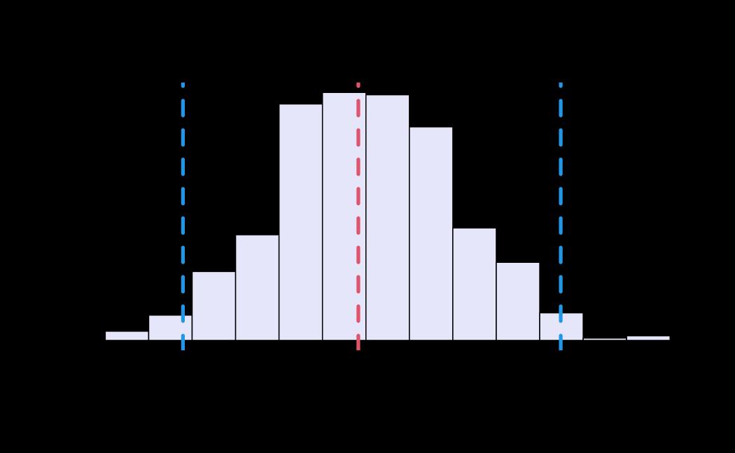
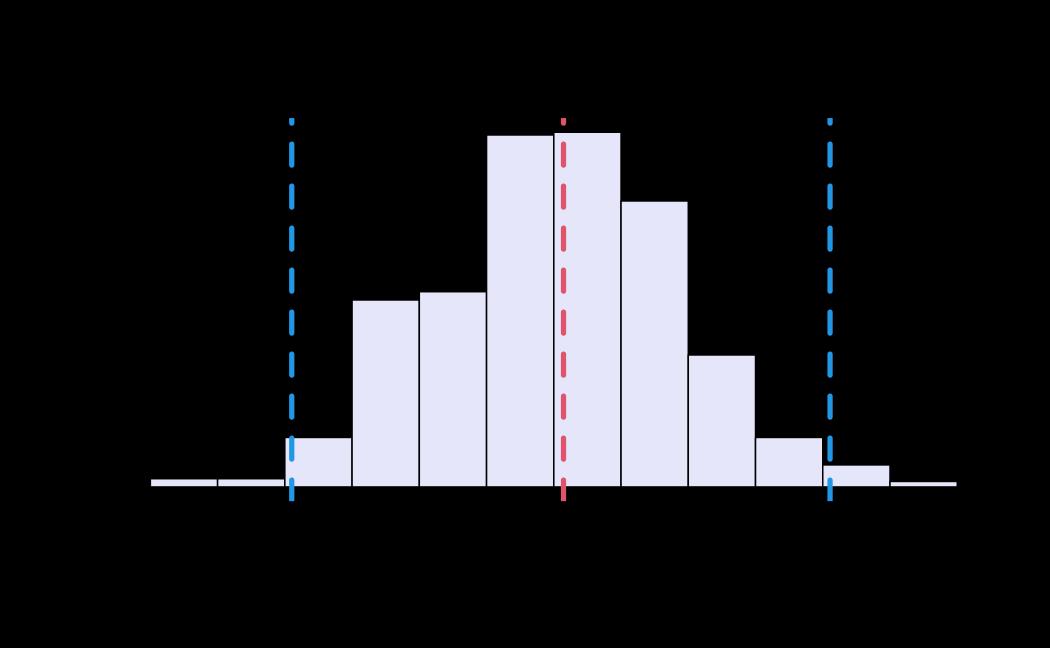
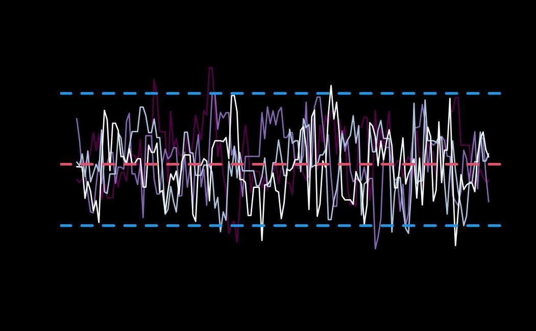
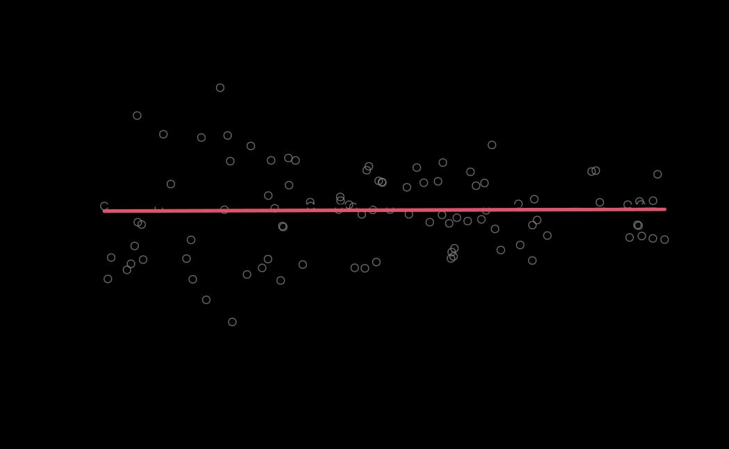
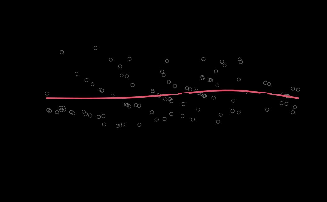
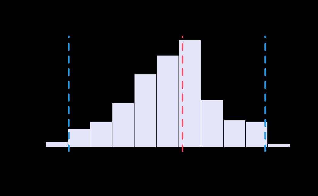
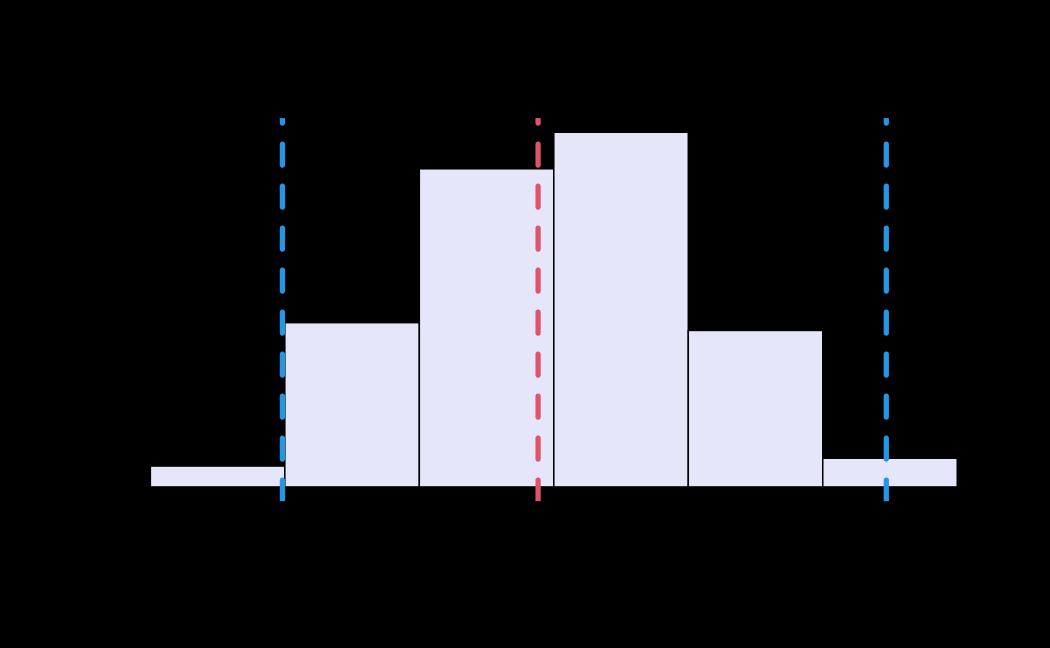
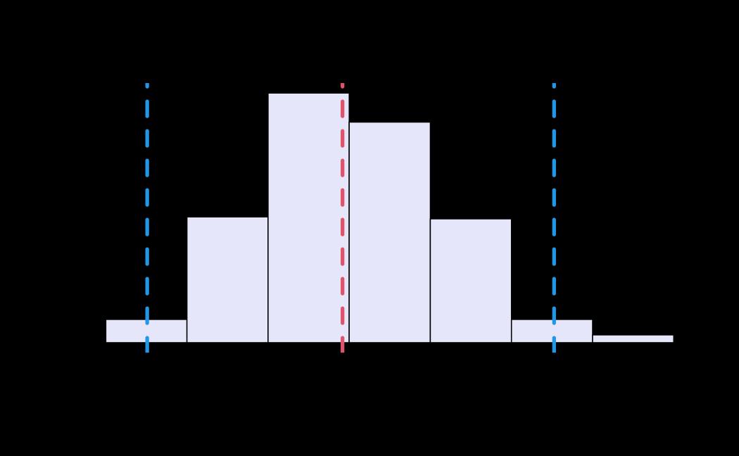
# plot (histograms and trace plot have highest posterior density intervals dashed lines in blue and posterior estimate in red)
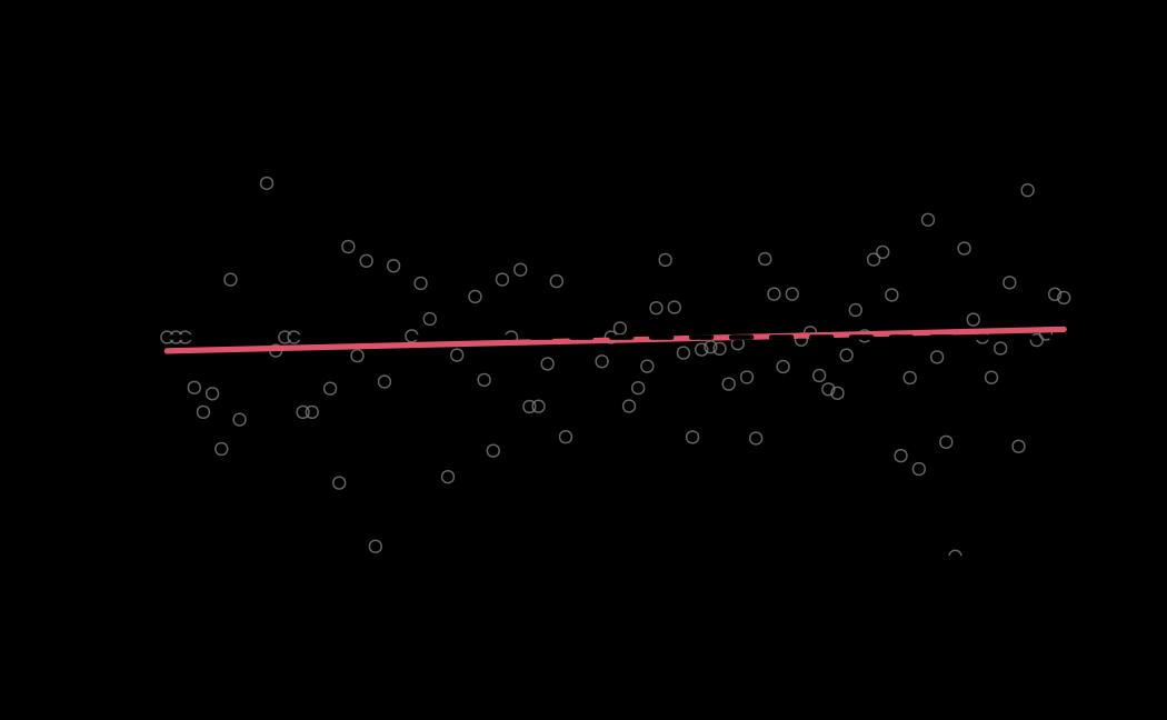
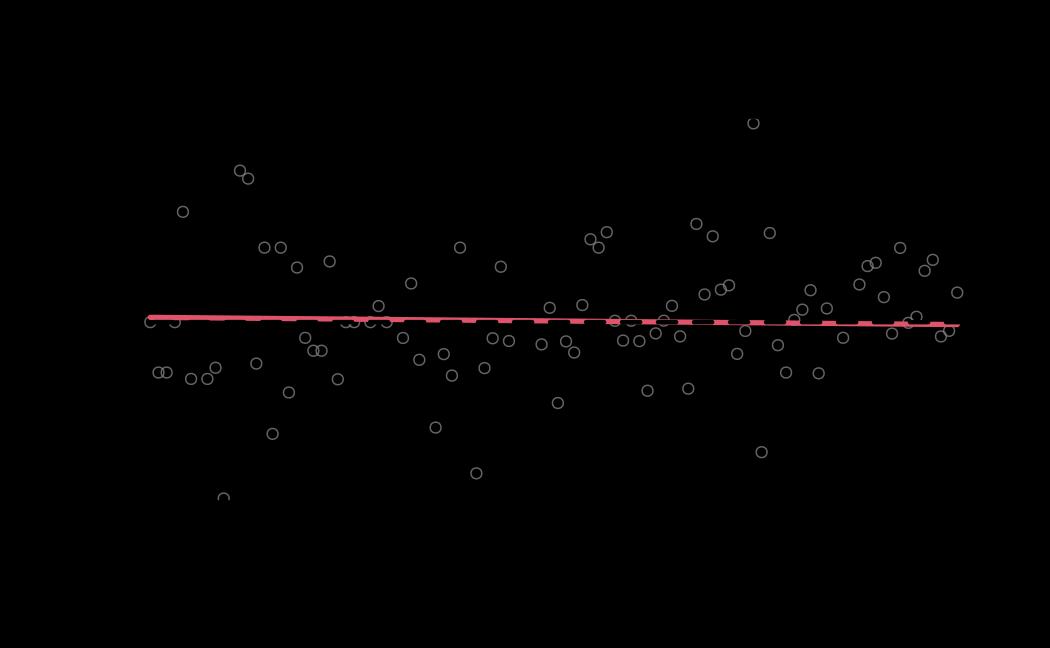
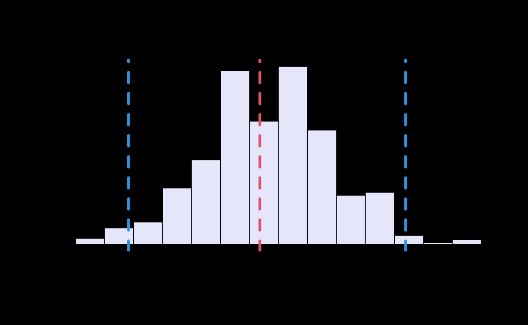
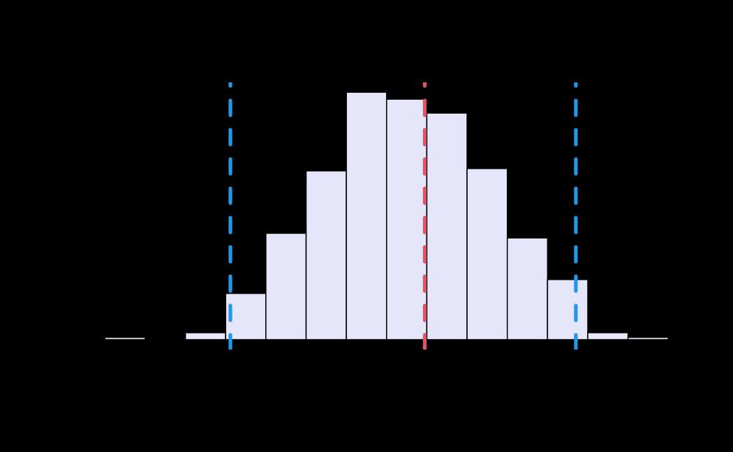
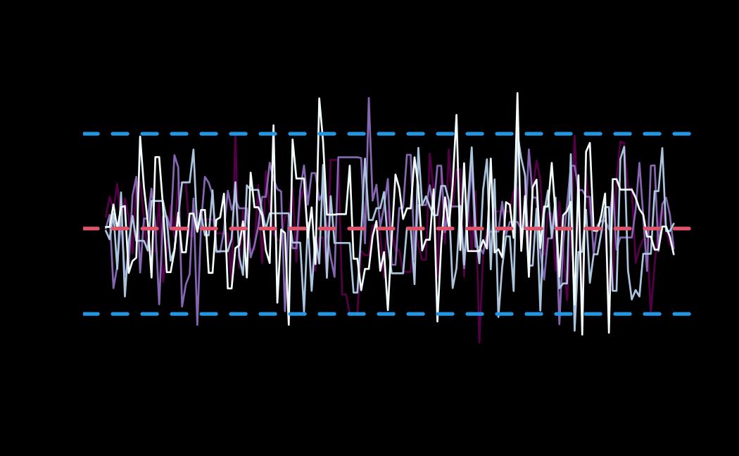
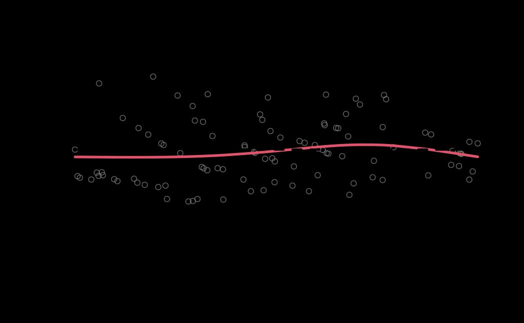
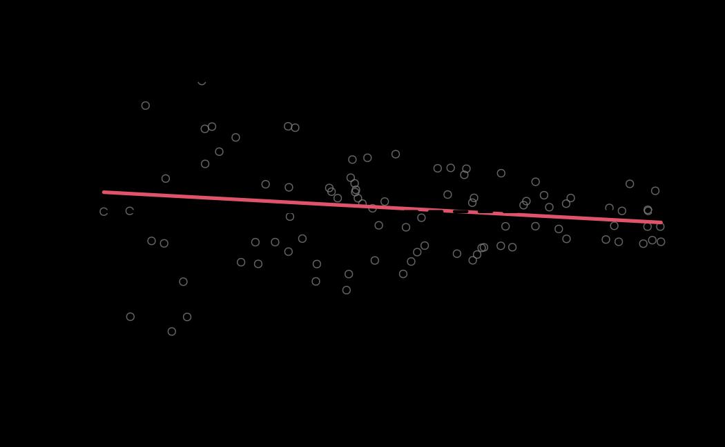
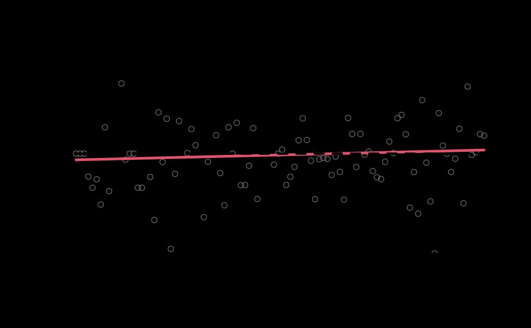
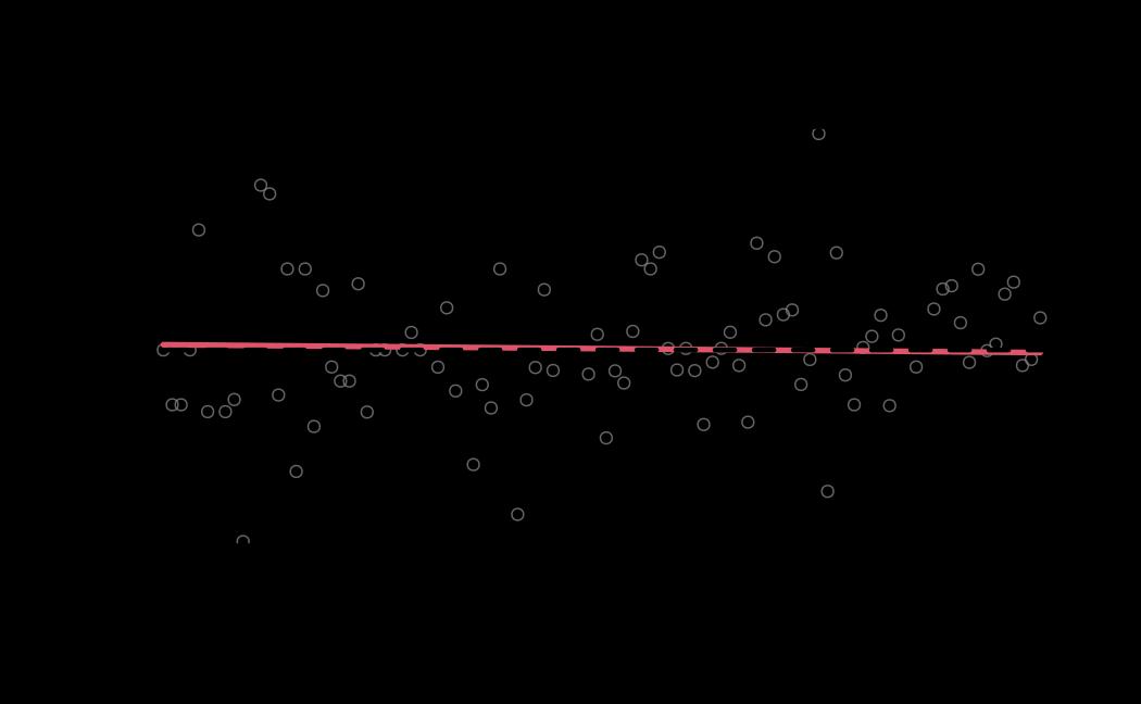
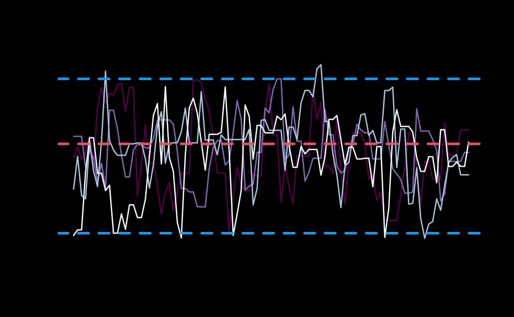
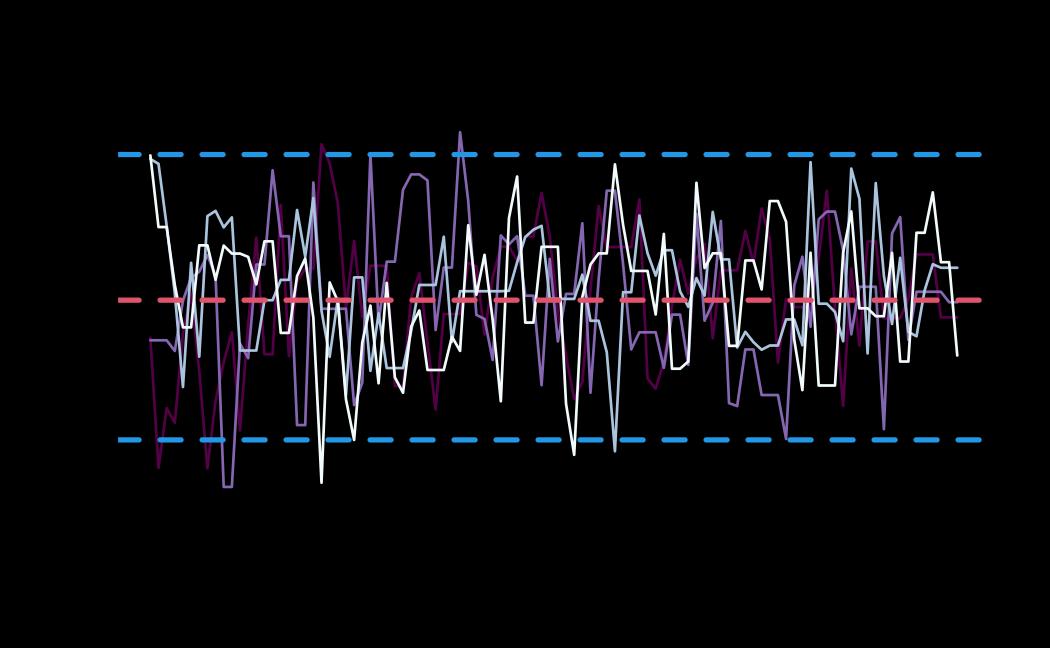
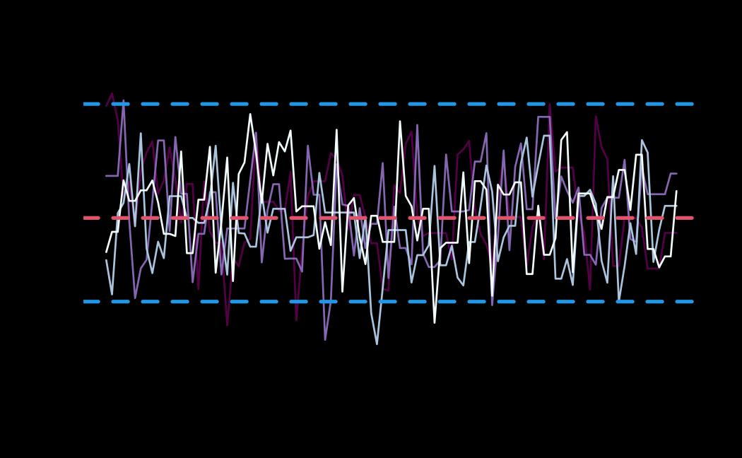
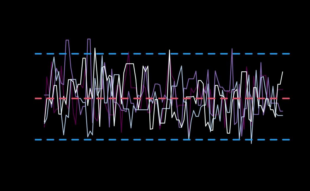
plot(x = tie_hmc, reh  = tie_reh, diagnostics = tie_hmc_diagnostics)

---

Actor-Oriented Modeling framework

For the actor-oriented modeling, we refer the modeling framework introduced by Stadtfeld and Block (2017), in which the process of realization of a relational event is described by two steps:

1. first the actor that is going to initiate the next interaction and becomes the “sender” of the future event;
2. then the choice of the “receiver” of the future event operated by the active “sender” in step 1.

The first step is modelled via a rate model (similar to a REM), in which the waiting times are modelled along with the sequence of the senders of the observed relational events. The second step is modelled via a multinomial discrete choice model, where we model the choice of the receiver of the next event conditional to the active sender at the first step.

Therefore, the two models can be described by two separate likelihood functions with their own set of parameters. The parameters in each model will describe the effect that explanatory variables (network dynamics and other available exogenous statistics) have on the two distinct processes. The estimation of the model parameters for each model can be carried out separately and for this reason, the user can also provide a remstats object containing the statistics of either both or one of the two models.

---

The likelihood function

Consider a time-ordered sequence of \(M\) relational events, \(E_{t_M}=(e_1,\ldots,e_M)\), where each event \(e_{m}\) in the sequence is described by the 3-tuple \((s_{m},r_{m},t_{m})\) (we exclude here the information about the event type), respectively sender, receiver, and time of the event. Furthermore, consider \(N\) to be the number of actors in the network. For simplicity, we assume that all actors in the network can be the sender or the receiver of a relational event (i.e. full risk set, see vignette(topic="riskset",package="remify") for more information on alternative definitions of the risk set) and we use the index \(n\) to indicate any actor in the set \(\mathcal{R}\) of actors at risk, thus \(n \in \left\lbrace 1,2,\ldots,N\right\rbrace\).

---

Sender activity rate model

The likelihood function that models the sender activity is:

\[ \mathscr{L}_{\text{sender model}}(\boldsymbol{\theta}; E_{t_M},X)= \prod_{m=1}^{M}{\Bigg[\tau(s_{m},t_{m},\boldsymbol{\theta})\prod_{n \in \mathcal{R}}^{}{\exp{\left\lbrace-\tau(n,t_{m},\boldsymbol{\theta})\left(t_m-t_{m-1}\right)\right\rbrace} }}\Bigg] \]

where:

• \(\tau(n,t_{m},\boldsymbol{\theta})\) is the activity rate of sender \(n\) at time \(t_{m}\). The sender activity rate describes the istantaneous probability that a sender initiates an interaction at a specific time point and it is modeled as \(\tau(n,t_{m},\boldsymbol{\theta}) = \exp{\left\lbrace \boldsymbol{\theta}^{T}X_{[m,n,.]}\right\rbrace}\) where:
  • \(\boldsymbol{\theta}\) is the vector of parameters of interest. Such parameters describe the effect that the sufficient statistics (explanatory variables) have on the activity rate of the sender;
  • \(\boldsymbol{\theta}^{T}X_{[m,n,.]} = \sum_{p=1}^{P}{\theta_p X_{[m,n,p]}}\) is the linear predictor of the sender \(n\) at time \(t_{m}\). The object \(X\) is a three dimensional array with number of rows equal to the number of unique time points (or events) in the sequence (see vignette(package="remstats") for more information about statistics calculated per unique time point or per observed event), number of columns equal to number of actors in the sequence (\(N\)), number of slices equal to the number of variables in the linear predictor (\(P\)).
• \(s_m\) refers to the sender of the event observed at time \(t_m\) and \(n\) refers to any actor that can be sender of an interaction at time \(t_m\);
• \(\mathcal{R}\) describes the set of actors at risk of initiating an interaction, becoming then the future sender of a relational event (the set also includes the actor that is sender of the event at time \(t_m\)). In this tutorial, the risk set of the sender model is assumed to be the full risk set, where all the actors in the network can be “the sender” of a relational event at any time point in the event sequence;
• \((t_{m}-t_{m-1})\) is the waiting time between two subsequent relational events.

If the time of occurrence of the events is not available and we know only their order of occurrence, then the likelihood function for the sender model reduces to the Cox proportional-hazard survival model (Cox 1972),

\[ \mathscr{L}_{\text{sender model}}(\boldsymbol{\theta}; E_{t_M},X)= \prod_{m=1}^{M}{\Bigg[\frac{\tau(s_{m},t_{m},\boldsymbol{\theta})}{\sum_{n\in \mathcal{R}}^{}{\tau(n,t_{m},\boldsymbol{\theta})}}}\Bigg] \]

---

Receiver choice model

The likelihood function that models the receiver choice is:

\[ \mathscr{L}_{\text{receiver model}}(\boldsymbol{\beta}; E_{t_M},X)=\prod_{m=1}^{M}{\Bigg[\frac{\exp{\left\lbrace\boldsymbol{\beta}^{T}U_{[m,r_m,.]}\right\rbrace}}{\sum_{n \in \mathcal{R} \setminus \left\lbrace s_m \right\rbrace }^{}{\exp{\left\lbrace\boldsymbol{\beta}^{T}U_{[m,n,.]}\right\rbrace}}}\Bigg]} \]

where:

• \(\exp{\left\lbrace\boldsymbol{\beta}^{T}U_{[m,r_m,.]}\right\rbrace} \backslash \sum_{n \in \mathcal{R} \setminus \left\lbrace s_m \right\rbrace }^{}{\exp{\left\lbrace\boldsymbol{\beta}^{T}U_{[m,n,.]}\right\rbrace}}\) is the conditional probability that the sender \(s_m\) active at time \(t_m\) chooses \(r_m\) as the receiver of the next interaction, and:
  • \(\boldsymbol{\beta}\) is the vector of \(K\) parameters of interest. Such parameters describe the effect that the sufficient statistics (explanatory variables) have on the choice of a receiver;
  • \(\boldsymbol{\beta}^{T}U_{[m,n,.]} = \sum_{k=1}^{K}{\beta_k U_{[m,n,k]}}\) is the linear predictor of the event at time \(t_{m}\) in which the sender is \(s_m\) and the receiver is any of the possible receivers, \(n\) with \(n \neq s_m\). The object \(U\) is a three dimensional array with number of rows equal to the number of events in the sequence (see vignette(package="remstats") for more information about statistics calculated per unique time point or per observed event), number of columns equal to number of actors (\(N\)), number of slices equal to the number of variables in the linear predictor (\(K\)).
• \(r_m\) refers to the receiver observed at time \(t_m\) and \(n\) refers to any actor that can be the receiver of the event at time \(t_m\) (excluding the sender at time \(t_m\))
• \(\mathcal{R}\) describes the set of actors at risk of becoming the receiver of the next interaction. In the case of the receiver model, the risk set composition changes over time because at each time point the actor that is currently the sender cannot be also the receiver of the interaction and is excluded from the set of potential receivers. In this tutorial, the risk set of the reiceiver model is assumed to be the full risk set where all actors (excluding the current sender at each time point) can be “the receiver” at any time point.

---

A toy example on the actor oriented modeling framework

Consider the data ao_data, that is a list containing a simulated relational event sequence where events were generated by following the two-steps process described in the section above. We are going to model the sender activity rate and the receiver choice as:

\[ \tau(n,t_{m},\boldsymbol{\theta}) = \exp{\left\lbrace \theta_{\text{intercept}} + \theta_{indegreeSender}\text{indegreeSender}(n,t_{m})\right\rbrace} \]

\[ \exp{\left\lbrace \boldsymbol{\beta}^{T}U_{[m,n,.]} \right\rbrace} = \exp{\left\lbrace \beta_{\text{inertia}}\text{inertia}(s_m,n,t_{m}) + \beta_{\text{reciprocity}}\text{reciprocity}(s_m,n,t_{m})\right\rbrace}\]

Furthermore, we know that true parameters quantifying the effect of the statistics (name in subscript next to the model parameters \(\theta\) and \(\beta\)) used in the generation of the event sequence are:

• for the sender model, \[\begin{bmatrix} \theta_{intercept} \\ \theta_{\text{indegreeSender}} \end{bmatrix} = \begin{bmatrix} -5.0 \\ 0.01 \end{bmatrix}\]
• for the receiver model \[\begin{bmatrix} \beta_{\text{inertia}} \\ \beta_{\text{reciprocity}} \end{bmatrix} = \begin{bmatrix} -0.1 \\ 0.03\end{bmatrix}\]

The parameters are also available as object within the list, ao_data$true.pars.

# setting `ncores` to 1 (the user can change this parameter)
ncores <- 1L

# loading data
data(ao_data)

# true parameters' values
ao_data$true.pars

## $rate_model
##      intercept indegreeSender 
##          -5.00           0.01 
## 
## $choice_model
##     inertia reciprocity 
##       -0.10        0.03

# processing event sequence with 'remify'
ao_reh <- remify::remify(edgelist = ao_data$edgelist, model = "actor")

# summary of the relational event network
summary(ao_reh)

## Relational Event Network
## (processed for actor-oriented modeling):
##  > events = 100
##  > actors = 5
##  > riskset = full
##  > directed = TRUE
##  > ordinal = FALSE
##  > weighted = FALSE
##  > time length ~ 2654 
##  > interevent time 
##       >> minimum ~ 0.8542 
##       >> maximum ~ 167.3494

Estimating a model with remstimate() in 3 steps

The estimation of a model can be summarized in three steps:

1. First, we define the linear predictor with the variables of interest, using the statistics available within remstats (statistics calculated by the user can be also supplied to remstats::remstats()).

# specifying linear predictor (for rate and choice model, with `remstats`)
rate_model <- ~ 1 + remstats::indegreeSender()
choice_model <- ~ remstats::inertia() + remstats::reciprocity()

2. Second, we calculate the statistics defined in the linear predictor with the function remstats::remstats() from the remstats package.

# calculating statistics (with `remstats`)
ao_stats <- remstats::remstats(reh = ao_reh, sender_effects = rate_model, receiver_effects = choice_model)

# the 'aomstats' 'remstats' object
ao_stats

## Relational Event Network Statistics
## > Model: actor-oriented
## > Computation method: per time point
## > Sender model:
##   >> Dimensions: 100 time points x 5 actors x 2 statistics
##   >> Statistics:
##       >>> 1: baseline
##       >>> 2: indegreeSender
## > Receiver model:
##   >> Dimensions: 100 events x 5 actors x 2 statistics
##   >> Statistics:
##       >>> 1: inertia
##       >>> 2: reciprocity

3. Finally, we are ready to run any of the optimization methods with the function remstimate::remstimate().

# for example the method "MLE"
remstimate::remstimate(reh = ao_reh,
                          stats =  ao_stats,
                          method = "MLE",
                          ncores = ncores)    

## Relational Event Model (actor oriented) 
## 
## Coefficients rate model **for sender**:
## 
##       baseline indegreeSender 
##   -4.806201529   -0.008363321 
## 
## Null deviance: 1177.625 
## Residual deviance: 1177.348 
## AIC: 1181.348 AICC: 1181.472 BIC: 1186.558
## 
## --------------------------------------------------------------------------------
## 
## Coefficients choice model **for receiver**:
## 
##     inertia reciprocity 
## -0.03250837  0.01828748 
## 
## Null deviance: 2.772589 
## Residual deviance: 277.0551 
## AIC: 281.0551 AICC: 281.1789 BIC: 286.2655

In the sections below, as already done with the tie-oriented framework, we show the estimation of the parameters using all the methods available and we also show the usage and output of the methods available for a remstimate object.

---

Frequentist approaches

Maximum Likelihood Estimation (MLE)

ao_mle <- remstimate::remstimate(reh = ao_reh,
                        stats = ao_stats,
                        ncores = ncores,
                        method = "MLE",
                        WAIC = TRUE, # setting WAIC computation to TRUE
                        nsimWAIC = 100) # number of draws for the computation of the WAIC set to 100            

print( )

# printing the 'remstimate' object 
ao_mle

## Relational Event Model (actor oriented) 
## 
## Coefficients rate model **for sender**:
## 
##       baseline indegreeSender 
##   -4.806201529   -0.008363321 
## 
## Null deviance: 1177.625 
## Residual deviance: 1177.348 
## AIC: 1181.348 AICC: 1181.472 BIC: 1186.558 WAIC: 1181.781 
## 
## --------------------------------------------------------------------------------
## 
## Coefficients choice model **for receiver**:
## 
##     inertia reciprocity 
## -0.03250837  0.01828748 
## 
## Null deviance: 2.772589 
## Residual deviance: 277.0551 
## AIC: 281.0551 AICC: 281.1789 BIC: 286.2655 WAIC: 280.5819

summary( )

# summary of the 'remstimate' object
summary(ao_mle)

## Relational Event Model (actor oriented) 
## 
## Call rate model **for sender**:
## 
##  ~1 + remstats::indegreeSender()
## 
## 
## Coefficients rate model (MLE with interval likelihood):
## 
##                   Estimate    Std. Err     z value Pr(>|z|) Pr(=0)
## baseline        -4.8062015   0.1832563 -26.2266709      0.0 <2e-16
## indegreeSender  -0.0083633   0.0159467  -0.5244534      0.6 0.8971
## Null deviance: 1177.625 on 100 degrees of freedom
## Residual deviance: 1177.348 on 98 degrees of freedom
## Chi-square: 0.2770484 on 2 degrees of freedom, asymptotic p-value 0.8706422 
## AIC: 1181.348 AICC: 1181.472 BIC: 1186.558 WAIC: 1181.781 
## -------------------------------------------------------------------------------- 
## 
## Call choice model **for receiver**:
## 
##  ~remstats::inertia() + remstats::reciprocity()
## 
## 
## Coefficients choice model (MLE with interval likelihood):
## 
##              Estimate  Std. Err   z value Pr(>|z|) Pr(=0)
## inertia     -0.032508  0.077037 -0.421983   0.6730 0.9015
## reciprocity  0.018287  0.071630  0.255305   0.7985 0.9064
## Null deviance: 2.772589 on 100 degrees of freedom
## Residual deviance: 277.0551 on 98 degrees of freedom
## Chi-square: -274.2826 on 2 degrees of freedom, asymptotic p-value 1 
## AIC: 281.0551 AICC: 281.1789 BIC: 286.2655 WAIC: 280.5819

Information Critieria

# aic
aic(ao_mle)

##   sender model receiver model 
##      1181.3481       281.0551

# aicc
aicc(ao_mle)

##   sender model receiver model 
##      1181.4718       281.1789

# bic 
bic(ao_mle)

##   sender model receiver model 
##      1186.5584       286.2655

#waic 
waic(ao_mle)

##   sender model receiver model 
##      1181.7813       280.5819

diagnostics( )

# diagnostics
ao_mle_diagnostics <- diagnostics(object = ao_mle, reh = ao_reh, stats = ao_stats)

plot( )

# plot
plot(x = ao_mle, reh  = ao_reh, diagnostics = ao_mle_diagnostics)

---

Adaptive Gradient Descent Optimization (GDADAMAX)

ao_gd <- remstimate::remstimate(reh = ao_reh,
                        stats =  ao_stats,
                        ncores = ncores,
                        method = "GDADAMAX",
                        epochs = 200L, # number of iterations of the Gradient-Descent algorithm
                        WAIC = TRUE, # setting WAIC computation to TRUE
                        nsimWAIC = 100) # number of draws for the computation of the WAIC set to 100     
# print 
ao_gd

## Relational Event Model (actor oriented) 
## 
## Coefficients rate model **for sender**:
## 
##       baseline indegreeSender 
##     -0.1688384     -0.1017067 
## 
## Null deviance: 1177.625 
## Residual deviance: 10066.19 
## AIC: 10070.19 AICC: 10070.32 BIC: 10075.4 WAIC: 10287.92 
## 
## --------------------------------------------------------------------------------
## 
## Coefficients choice model **for receiver**:
## 
##     inertia reciprocity 
## -0.02370260  0.01567611 
## 
## Null deviance: 2.772589 
## Residual deviance: 277.0683 
## AIC: 281.0683 AICC: 281.192 BIC: 286.2787 WAIC: 280.3747

# diagnostics
ao_gd_diagnostics <- diagnostics(object = ao_gd, reh = ao_reh, stats = ao_stats)
# plot
# plot(x = ao_gd, reh  = ao_reh, diagnostics = ao_gd_diagnostics) # uncomment to use the plot function

---

Bayesian approaches

Bayesian Sampling Importance Resampling (BSIR)

library(mvnfast) # loading package for fast simulation from a multivariate Student t distribution
priormvt <- mvnfast::dmvt # defining which distribution we want to use from the 'mvnfast' package
ao_bsir <- remstimate::remstimate(reh = ao_reh,
                        stats =  ao_stats,
                        ncores = ncores,
                        method = "BSIR",
                        nsim = 100L, # 100 draws from the posterior distribution
                        prior = list(sender_model = priormvt, receiver_model = priormvt), #  defining prior here, prior parameters follow below
                        prior_args = list(sender_model =  list(mu = rep(0,dim(ao_stats$sender_stats)[3]), # prior mu value for sender_model
                                                            sigma = diag(dim(ao_stats$sender_stats)[3])*1.5, # prior sigma value for sender_model
                                                            df = 1),  # prior df value
                                        receiver_model = list(mu = rep(0,dim(ao_stats$receiver_stats)[3]), # prior mu value for receiver_model
                                                            sigma = diag(dim(ao_stats$receiver_stats)[3])*1.5, # prior sigma value for receiver_model
                                                            df = 1)), # prior df value
                        log = TRUE, # requiring log density values from the prior,
                        seed = 20929, # set a seed only for reproducibility purposes
                        WAIC = TRUE, # setting WAIC computation to TRUE
                        nsimWAIC = 100 # number of draws for the computation of the WAIC set to 100     
                        )

# summary 
summary(ao_bsir)

## Relational Event Model (actor oriented) 
## 
## Call rate model **for sender**:
## 
##  ~1 + remstats::indegreeSender()
## 
## 
## Posterior Modes rate model (BSIR with interval likelihood):
## 
##                 Post.Mode    Post.SD      Q2.5%       Q50%  Q97.5% Pr(=0|x)
## baseline       -4.8018252  0.1759390 -5.0995898 -4.7823997 -4.4837   <2e-16
## indegreeSender -0.0080396  0.0161221 -0.0390818 -0.0071234  0.0230   0.8983
## Log posterior: -588.6755 WAIC: 1181.684 
## -------------------------------------------------------------------------------- 
## 
## Call choice model **for receiver**:
## 
##  ~remstats::inertia() + remstats::reciprocity()
## 
## 
## Posterior Modes choice model (BSIR with interval likelihood):
## 
##              Post.Mode    Post.SD      Q2.5%       Q50% Q97.5% Pr(=0|x)
## inertia     -0.0126845  0.0811262 -0.1744974 -0.0077218 0.1423   0.9081
## reciprocity  0.0198576  0.0751748 -0.1140912  0.0010799 0.1581   0.9062
## Log posterior: -138.4584 WAIC: 282.0644

# diagnostics
ao_bsir_diagnostics <- diagnostics(object = ao_bsir, reh = ao_reh, stats = ao_stats)
# plot (only for the receiver_model, by setting sender_model = NA)
# plot(x = ao_bsir, reh  = ao_reh, diagnostics = ao_bsir_diagnostics, sender_model = NA) # uncomment to use the plot function

---

Hamiltonian Monte Carlo (HMC)

ao_hmc <- remstimate::remstimate(reh = ao_reh,
                        stats =  ao_stats,
                        method = "HMC",
                        ncores = ncores,
                        nsim = 300L, # 300 draws to generate per each chain
                        nchains = 4L, # 4 chains (each one long 200 draws) to generate
                        burnin = 300L, # burnin length is 300
                        L = 100L, # number of leap-frog steps
                        epsilon = 0.1/100, # size of a leap-frog step
                        thin = 2L, # thinning size (this will reduce the final length of each chain will be 150)
                        seed = 23029, # set a seed only for reproducibility purposes
                        WAIC = TRUE, # setting WAIC computation to TRUE
                        nsimWAIC = 100 # number of draws for the computation of the WAIC set to 100     
                        )

# summary 
summary(ao_hmc)

## Relational Event Model (actor oriented) 
## 
## Call rate model **for sender**:
## 
##  ~1 + remstats::indegreeSender()
## 
## 
## Posterior Modes rate model (HMC with interval likelihood):
## 
##                 Post.Mode    Post.SD      Q2.5%       Q50%  Q97.5% Pr(=0|x)
## baseline       -4.6587527  0.1024161 -4.8466379 -4.6503193 -4.4549   <2e-16
## indegreeSender -0.0192776  0.0090939 -0.0372322 -0.0195099 -0.0029   0.5139
## Log posterior: -599.8593 WAIC: 1179.536 
## -------------------------------------------------------------------------------- 
## 
## Call choice model **for receiver**:
## 
##  ~remstats::inertia() + remstats::reciprocity()
## 
## 
## Posterior Modes choice model (HMC with interval likelihood):
## 
##              Post.Mode    Post.SD      Q2.5%       Q50% Q97.5% Pr(=0|x)
## inertia     -0.0328733  0.0440346 -0.1198729 -0.0259082 0.0533   0.8833
## reciprocity  0.0189472  0.0410635 -0.0669650  0.0092633 0.0905   0.8999
## Log posterior: -138.5283 WAIC: 278.4279

# diagnostics
ao_hmc_diagnostics <- diagnostics(object = ao_hmc, reh = ao_reh, stats = ao_stats)
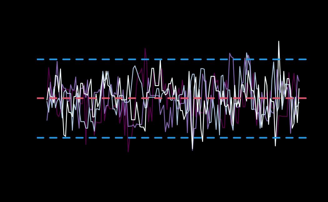
# plot (only for the receiver_model, by setting sender_model = NA)
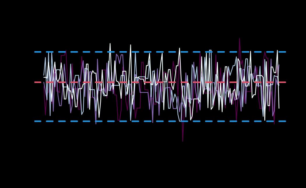
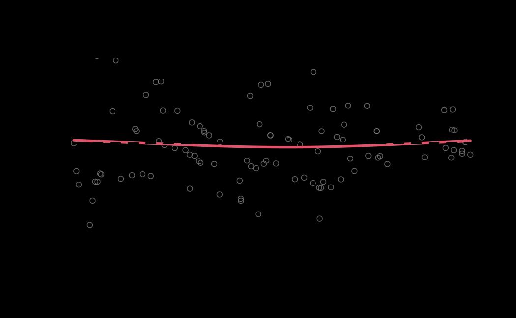
plot(x = ao_hmc, reh  = ao_reh, diagnostics = ao_hmc_diagnostics, sender_model = NA)

---

References

Butts, Carter T. 2008. “4. A Relational Event Framework for Social Action.” Sociological Methodology 38 (1): 155–200. https://doi.org/10.1111/j.1467-9531.2008.00203.x.

Cox, D. R. 1972. “Regression Models and Life-Tables.” Journal of the Royal Statistical Society. Series B (Methodological) 34 (2): 187–220. http://www.jstor.org/stable/2985181.

Stadtfeld, Christoph, and Per Block. 2017. “Interactions, Actors, and Time: Dynamic Network Actor Models for Relational Events.” Sociological Science 4 (14): 318–52. https://doi.org/10.15195/v4.a14.