This vignette provides a definition of full,
active and manual risk set, it explains how a
manual risk set is declared in the processing function
remify::remify(), and it shows how the processed risk set
looks like in the remify object.
Consider the remify object for the network
randomREHsmall.
library(remify) # loading package
data(randomREHsmall) # data

# processing the edgelist
reh <- remify(edgelist = randomREHsmall$edgelist,
                          directed = TRUE, # events are directed
                          ordinal = FALSE, # model with waiting times
                          model = "tie", # tie-oriented modeling
                          actors = randomREHsmall$actors,
                          origin = randomREHsmall$origin,
                          omit_dyad = NULL)

# summary(reh)
Definition of risk set
A relational event history consists of a time-ordered sequence of (directed or undirected) interaction. For each event, we know:
- its time of occurrence, either as timestamp/date/continuous value or just as order
- the actors that were involved in the realtional event
- the type of the event (if measured)
For instance, the first five events of the
randomREHsmall sequence are reported as follows
randomREHsmall$edgelist[1:5,]## time actor1 actor2
## 1 2020-03-05 15:36:37 Colton Kayla
## 2 2020-03-05 18:34:11 Lexy Colton
## 3 2020-03-05 19:49:37 Colton Kayla
## 4 2020-03-05 20:38:23 Colton Kayla
## 5 2020-03-06 05:54:12 Richard Coltonwhere time, actor1, actor2
describe each observed event in the sequence (Note that in this example
the type of events is not annotated).
When modeling a relational event sequence, we have to define per each
time point a risk set, which consists of the set of those relational
events (dyads) that at a specific time point were likely to be observed
(this set also contains the event that is actually observed at a
specific time point). The definition of the risk set is an important
building block of the likelihood function for both tie-oriented and
actor-oriented modeling framework. In the sections of this vignette, we
discuss three possible definitions of the risk set: full,
active and manual risk set. These three types of risk
set can be processed with remify::remify() by specifying
the risk set type to the input argument riskset.
The full risk set
The most common definition of the risk set assumes that all the
possible dyads are likely to occur over the whole observation period. We
refer to this definition as full risk set. If the network has
N actors and it consists of directed events that can assume a
number of C possible event types, then the risk set will be
characterized by all the possible directed dyads among N
actors, which are D = N(N-1)C, or D = N(N-1)C/2 in the
case of undirected dyads. For instance, in the random network
(randomREHsmall) dyads are directed, actors are N =
5 and event types are C = 1, therefore we expect the
dimension of the risk set to be D = 5 * 4 * 1 = 20. The first
five dyads in the full risk set will be
##   dyadID    actor1    actor2
## 1      1    Colton Francesca
## 2      2    Colton     Kayla
## 3      3    Colton      Lexy
## 4      4    Colton   Richard
## 5      5 Francesca    Colton
The ID of the dyads (dyadID) corresponds to the order of
the dyads used by the functions in
`and it is processed by the functionremify::remify()`. The
ID of the dyads is defined by a two-steps approach:
- Actors’ and types’ names are first sorted according to their
alphanumericorder, that for the actors in the random network will be,
The alphanumeric order follows first the order of numbers from 0 to 9, then the alphabetical order of the letters.
For instance, given the vector of names
c("user22","0usr","1user","1deer"), its alphanumeric order will bec("0usr","1deer","1user","user22)
# sorted vector of actors' names
sorted_actors <- sort(randomREHsmall$actors)
sorted_actors
## [1] "Colton" "Francesca" "Kayla" "Lexy" "Richard"
# number of actors in the network
N <- length(randomREHsmall$actors)
and for the event type will be
# no event type, we set it to an empty string
sorted_types <- c(" ")

# C = 1 for 'randomREHsmall'
C <- length(sorted_types)
In this phase, the processing function remify::remify()
will also assign numeric IDs to both actors and event types
# IDs of actors will consist of an integer number from 1 to N
names(sorted_actors) <- 1:N
sorted_actors
## 1 2 3 4 5
## "Colton" "Francesca" "Kayla" "Lexy" "Richard"
# IDs of types will be an integer number from 1 to C
names(sorted_types) <- 1:C # in this case is one (artificial) event type
sorted_types
## 1
## " "- dyads are defined by the triple
c(actor1,actor2,type)that is found by looping first onactor2, thenactor1, and finallytype. An example of the loops is shown below
# initializing matrix object where to store the dyads as [actor1,actor2,type]
dyad_mat <- matrix(NA, nrow = N*(N-1)*C, ncol = 3)
colnames(dyad_mat) <- c("actor1","actor2","type")
rownames(dyad_mat) <- 1:(N*(N-1)*C)

# initializing position index
d <- 1

# start three loops
for(type in sorted_types){ # loop over event types,
  for(actor1 in sorted_actors){ # loop over actor1
    for(actor2 in sorted_actors){ # loop over actor2
      if(actor1!=actor2){ # avoid self-loops
        dyad_mat[d,] <- c(actor1,actor2,type)
        d <- d + 1
      }
    }
  }
}

 # same result as showed above by using the method `getDyad()`
dyad_mat[1:5,]
## actor1 actor2 type
## 1 "Colton" "Francesca" " "
## 2 "Colton" "Kayla" " "
## 3 "Colton" "Lexy" " "
## 4 "Colton" "Richard" " "
## 5 "Francesca" "Colton" " "
# checking the size of the _full_ risk set that is 20
dim(dyad_mat)[1]
## [1] 20The matrix dyad_mat above describes the full
risk set and the row indices correspond to the ID of each dyad
(dyadID). For instance, the dyadID is useful
in the case of tie-oriented modeling, where the remify
object will contain the attribute named "dyad", which
describes the time-ordered sequence of ID’s as to the observed
dyads.
# accessing the first values of the attribute "dyad"
# (attribute available only for tie-oriented modeling)
head(attr(reh,"dyad"))
## [1] 2 13 2 2 17 2Visualizing the risk set
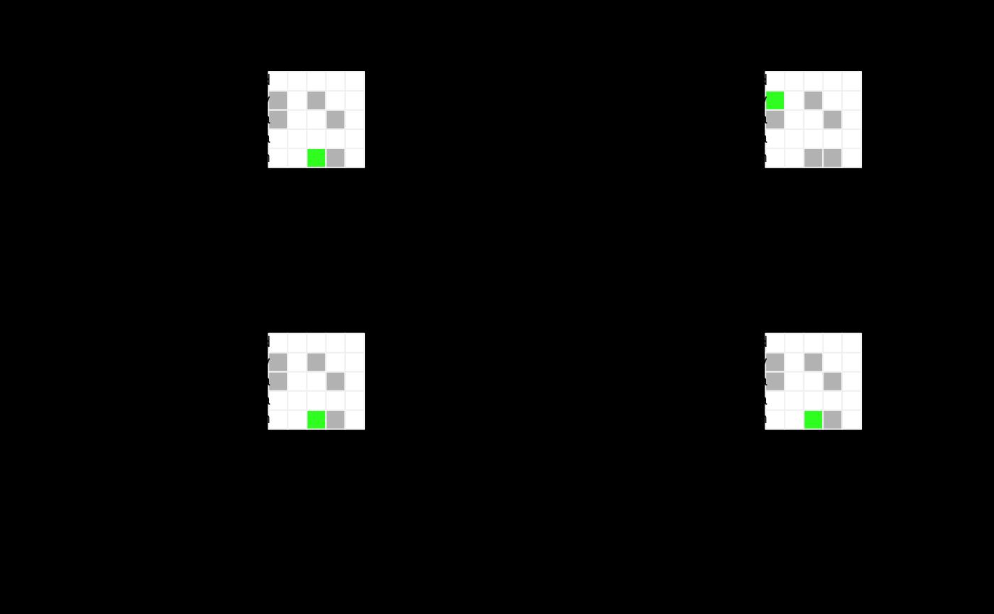
A possible way for visualizing the risk set composition at each time point consists in plotting a grid with actors’ names on both axes: referring to the senders (on the y-axis) and to the receivers (on the x-axis).

Cosidering the first four time points of randomREHsmall,
we observe: the (directed) dyad (Colton,Kayla) at time
,
and
and the (directed) dyad (Lexy,Colton) at time
.
The cell corresponding to the relational event occurred at each time
point is colored in green. The rest of the cells are colored in gray,
indicating those dyadic events that could have occurred and they are
part of the risk set. Cells in white, indicate those events that could
not occur (in this case the self-loops, like (Colton,Colton),
where sender and receiver are the same actor).
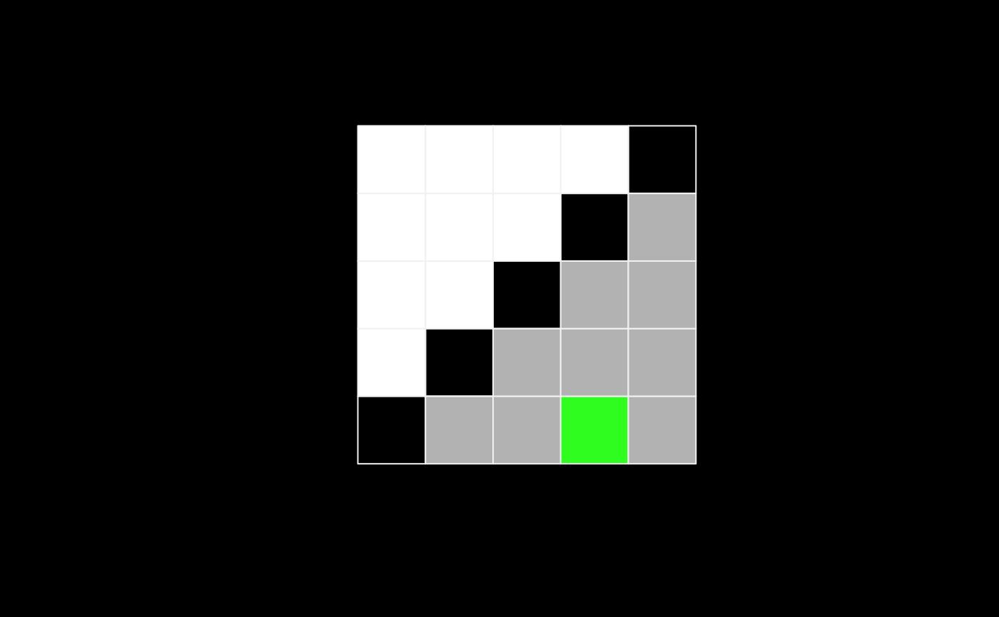
A full risk set in undirected networks will assume a
particular grid visualization. The dyads at risk will be on the lower
triangular grid, because the actor names c(actor1,actor2)
describing the dyad in the input edgelist are sorted according to their
alphanumeric order before being processed. For instance, the event at
c("Lexy","Colton"), will be rearranged as
c("Colton","Lexy"), and the risk set will change as follows
in the picture below.

The active and manual risk set
A full risk set is assumed to have a constant structure throughout the whole event history. All the possible dyads are assumed to be always at risk regardless any consideration about: (i) the possibility of one or more actors to still be able to interact with the other actors during the observation period, (ii) the possiblity of some event types to actually occur.
From this observation, the concept of a risk set structure that
changes over time may accomodate certain relational event histories in
which, actors, dyads or event types may not be observed within
prespecified time windows. Two alternative definitions of the risk set
can be declared with remify::remify():
- the active risk set, which reduces its size to only the dyadic events that are observed across the event history and it mantains the same (modified) structure over time
- the manual riskset, which allows the user to specify a more flexible risk set with a time-varying structure, in which actor, dyads or event types can be excluded at specific time intervals of the event history.
The active risk set
There exist relational event networks that have a large number of actors and the number of observed dyads is by far lower than the potential number of dyads (i.e. the size of the full risk set).
A measure of global density can be calculated over the whole event
sequence as the ratio
,
where
is the number of observed dyadic events and it can vary between
and
.
When a very low portion of dyads takes action in the network, we can
think of restricting the risk set only to such observed dyads. This risk
set reduction leads to the active risk set, which mantains the
same structure over time but is restricted to the dyads that were
observed at least one time in the event history. This type of risk set
can be declared by specifying riskset = "active" in
remify::remify()
The use of the active risk set can significantly decrease the computational time of both the calculation of statistics and the estimation of model parameters. However, the reduction of the risk set to the set of active (observed) dyads causes the exclusion of dyadic events that perhaps should be still included in the risk set. It is always good practice to explore the set of active dyads and take the due considerations given the type of data at hand, for instance: (i) expecting potential biases coming from the definition of an active risk set, (ii) considering to define a modification of the active risk set that avoids the exclusion of a set of additional actors/dyads/event types from the risk set even if they were not observed in the event history.
The manual risk set
There are circumstances in which one or more actors cannot take part in a relational event or an event type cannot be observed. This can happen either for a time window that can assume one of the following definitions:
- the time window is embedded in the event history, e.g., some actors temporarily drop the network
- the time window starts from a time point after the start of the event history and stops with the end of the history, e.g., when actors leave the network without poissibility of return
- the time window starts with beginning of the event history and stops before the end of the study, e.g., actors that join the network after the beginning of the event history and could only interact after they join.
To give a grasp of a few possible real scenarios in which actors/dyads/event types may be excluded from the risk set, we introduce three examples:
Example 1: when the relational event network is about in-person interactions (e.g., at the university or at school) and it is measured over days (or even weeks or months). One or more actors may not be present during one or more days, therefore we want to exclude such actors from the risk set for the specific time spans in which they could not interact. Furthermore, one or more actors may join (leave) the network after (before) the beginning (end) of the event history and this can also define specific restrictions on the risk set for such actors.
Example 2: when relational events are observed at a conference where multiple sessions or workshops can occur at the same time. In this case, the set of dyads at risk reduces to smaller different risk sets, each one based on the groups of actors participating at a specific session or workshop (constraints on the risk set here apply as a response to spatial constraints during a sesison or a workshop).
Example 3: when the relational events are digital interactions and one or more actors cannot interact one another because they do not appear in each other’s friends list (which may be a requirement in order to be able to interact).
In such scenarios and in many others, a full risk set would account for relational events that are not feasible and this may even lead to biased estimates of the model parameters. On contrary, it is possible to account for changes of the risk set over time by defining a manual risk set.
A manual risk set consists of a time-based definition of the
ensemble of dyads at risk where the user specifies which dyads to remove
from the full risk set at a specific time interval of the
study. This can be done via the omit_dyad argument of the
function remify::remify(). The user can define multiple
modifications of the full risk set occurring at different, or
even overlapping, time windows. In each modification, the user specifies
the set of actors, or dyads, or event types to be omitted.
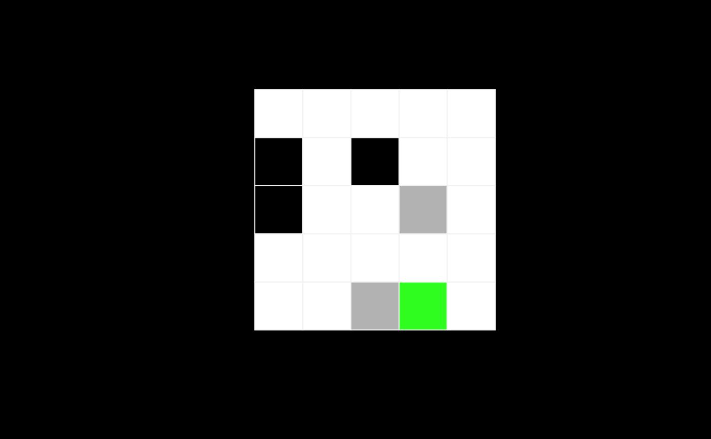
Consider the first four time points of the small random network and
assume this time that actors "Richard" and
"Francesca" didn’t join the study until the second day of
the study. This means that the risk set for at least the first four time
points will have the following composition,

where the tiles defining the dyads where "Richard" and
"Francesca" are either the sender (actor1) or receiver
(actor2) are excluded from the risk set (the tiles are now in white).
The risk set is now made of only those dyads in which
"Colton", "Kayla" and "Lexy"are
either the sender or the receiver of a relational event (tiles in
gray).
Finally, a manual risk set can be defined also for
undirected networks and the grid visualization will focus on the lower
triangular grid, because the actor names c(actor1,actor2)
describing the dyad in the input edgelist are sorted according to their
alphanumeric order by the processing. For instance, the event at
c("Lexy","Colton"), will be rearranged as
c("Colton","Lexy"), thus the risk set will change as
below.

Specifying a manual risk set: the
omit_dyad argument
The input argument omit_dyad is required when the
argument riskset = "manual". With this argument, the user
describes the time windows and the actor/dyads/event types to exclude
from them. The object to supply via the argumen omit_dyad
consists of a list of modifications. Each list refers to one risk set
modification and must be a list of two objects: a
data.frame called dyad, where dyads to be
removed are specified by row in the format
actor1, actor2, type, and a vector called time
which describes the first and last time point of the time window where
to apply the modification.
Example on five risk set modifications
Consider the randomREH data.
data(randomREH)For instance, we want to modify (reduce) the risk set according to five changes that apply on different time intervals:
- an event type
conflictthat was no more feasible since a specific time point until the end of the observation period.
randomREH$omit_dyad[[1]]$time # start and stop time point defining the time window of interest## [1] "2020-05-07 20:42:38 UTC" "2020-05-23 21:46:41 UTC"
randomREH$omit_dyad[[1]]$dyad # dyads to be removed from the time points defined by the interval in `time`## actor1 actor2 type
## 1 NA NA conflict- two actors
MichaelaandZackarythat couldn’t interact with anybody else after a specific time point until the last observed time point.
randomREH$omit_dyad[[2]]$time## [1] "2020-05-19 23:30:09 UTC" "2020-05-23 21:46:41 UTC"
randomREH$omit_dyad[[2]]$dyad## actor1 actor2 type
## 1 Michaela <NA> NA
## 2 <NA> Michaela NA
## 3 Zackary <NA> NA
## 4 <NA> Zackary NAThe object dyad will give instructions such that the
function will remove from the risk set at the indicated time windows all
the events where: (1) type is conflict, (2)
Michaela and `Zackary are senders or
receivers.
In this example we also add three more modifications of the risk set
that are not present in the object randomREH$omit_dyad but
that allow to explain how the input omit_dyad works, and
also how the processed risk set object will look like (in the next
section):
- actors
Maya,Alexander,RichardandCharlesjoined the network after the start of the event history.
randomREH$omit_dyad[[3]]$time ## [1] NA "2020-04-02 03:31:13 UTC"
randomREH$omit_dyad[[3]]$dyad ## actor1 actor2 type
## 1 Maya <NA> NA
## 2 Alexander <NA> NA
## 3 Richard <NA> NA
## 4 Charles <NA> NA
## 5 <NA> Maya NA
## 6 <NA> Alexander NA
## 7 <NA> Richard NA
## 8 <NA> Charles NA- actor
Breannaleft the network during a long time interval (about 2 months) embedded in the event history.
randomREH$omit_dyad[[4]]$time## [1] "2020-03-27 09:55:56 UTC" "2020-05-13 10:17:57 UTC"
randomREH$omit_dyad[[4]]$dyad## actor1 actor2 type
## 1 Breanna <NA> NA
## 2 <NA> Breanna NA- actor
Meganleft the network for a few days.
randomREH$omit_dyad[[5]]$time## [1] "2020-04-30 07:44:08 UTC" "2020-05-04 01:20:53 UTC"
randomREH$omit_dyad[[5]]$dyad## actor1 actor2 type
## 1 Megan <NA> NA
## 2 <NA> Megan NA
Using NA values to remove sets of
actors/dyads/event types
The <NA> values mean that all the actors/event
types are considered in that field. Indeed, in the change 1. where we
needed to remove all the events where conflict was the
type, we did it by leaving both actor1 and
actor2 unspecified <NA>. Therefore,
every time one of the fields among
(actor1,actor2,type) is left
undefined, the reduction applies to all the possible values of that
field. Another example are the risk set chages declared in 4. and 5.,
where we wanted to exclude all the dyads in which Breanna
and Megan are either the sender or the receiver of a
relational event. Therefore, we defined a data.frame named
"dyad" with two rows: one row in which
Breanna(Megan) appeared as the sender, and a
second row in which Breanna (Megan) appeared
as the receiver. We left the other fields set to NA,
meaning that (by row) all the possible event types and actors are to be
considered.
The processed risk set
The function remify::remify() processes the list of
modifications supplied to omit_dyad (only when
riskset = "manual"). The aim is to elaborate the risk set
modifications by accounting for the possible partial/complete
overlapping of time windows. A way to understand whatthe processing does
is to consider the plot of the input modifications and show the plot of
the final processing.
edgelist_reh <- remify::remify(edgelist = randomREH$edgelist,
                    directed = TRUE, # events are directed
                    ordinal = FALSE, # model with waiting times
                    model = "tie", # tie-oriented modeling
                    actors = randomREH$actors,
                    types = randomREH$types,
                    riskset = "manual",
                    origin = randomREH$origin,
                    omit_dyad = randomREH$omit_dyad)
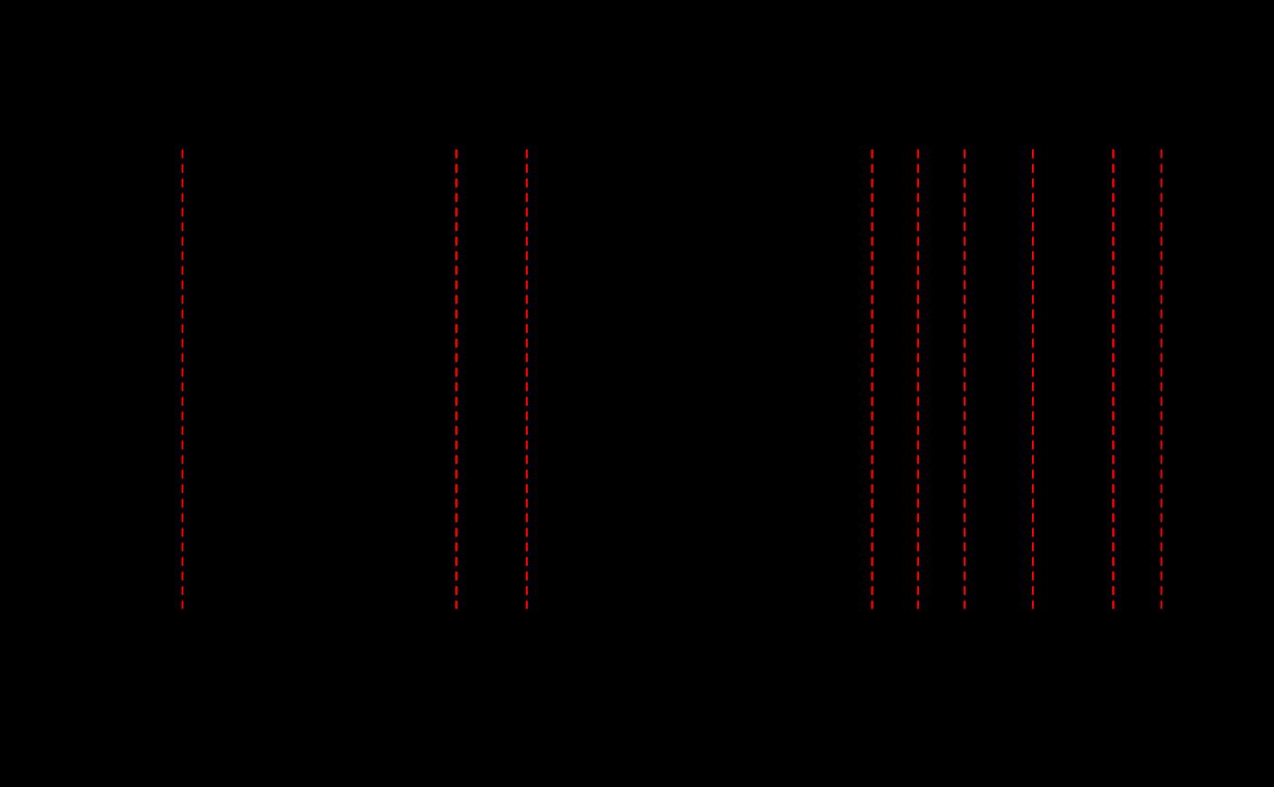
The processing function understands the partial/complete overlapping
of the time windows and defines new time intervals in which one or more
risk set changes are observed. In the plot below, the vertical
boundaries (dashed red lines) indicate the time intervals. Such time
bounds are used from the processing function to intersect the time
windows decalred in omit_dyad and define new time
intervals, where the changes of the risk set are processed according to
the new time windows. If the user supplies time windows that are not
overlapping, then the processed risk set will have the same structure of
the input.

After the processing of a relational event history, the
remify object will contain a list called
omit_dyad where two objects (time and
riskset) will describe the processed risk set
modifications. As a result of the processing of the five risk set
modifications, the risk set is describe now by eight risk set
modifications. This is due to the partial/total overlapping of two or
more time intervals. For instance, the second modification of the
processed risk set (figure below) will contain the combination of the
third and the fourth modification declared in the input
omit_dyad (figure above).

